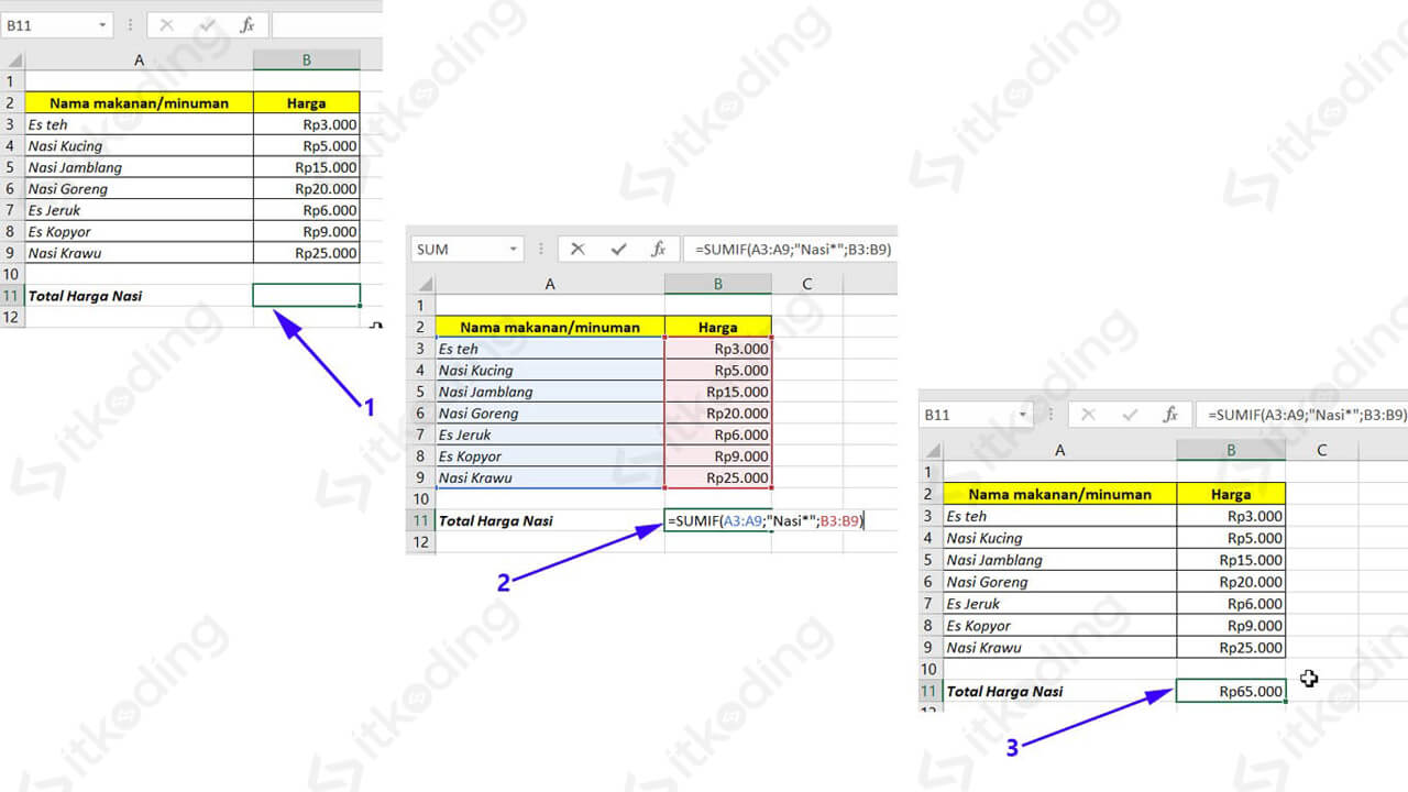
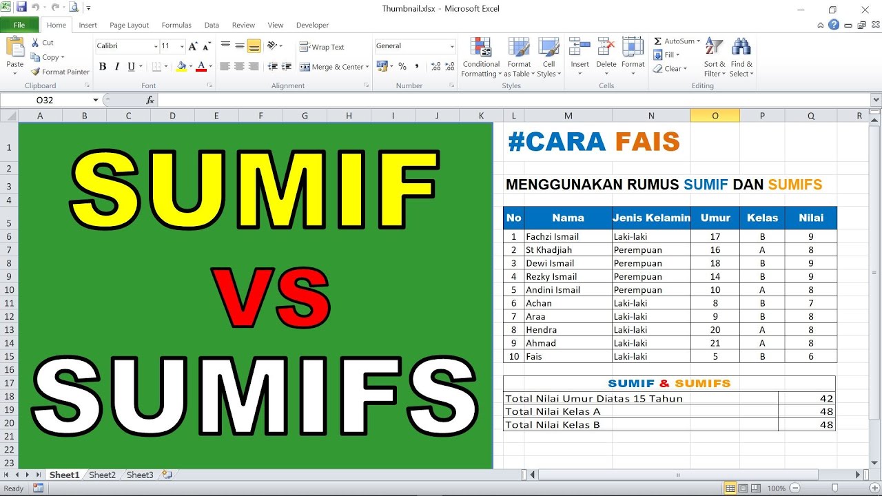
Rumus SUMIF Excel (Cara dan Contoh Fungsi SUMIF di Excel)
I have a data range in my w/sheet KK2:KR100. I am trying to sum values from this range on two column criteria. Criteria 1> KL2:KL100 text values.> Match text value wildcard characters = "BOI"> match "BOI" text value from range KL2:KL100 and sum numerical values from KO2:KO100 range and Criteria 2 > KR2:KR100 also having text values > Text value to be matched from this range is > "CAWD" > match.
SUMIFS with multiple criteria and OR logic Excel formula Exceljet
Video ini menjelaskan caranya menjumlahkan data di Excel dengan 2 kriteria. Kita akan menggunakan rumus SUMIFS. FILE LATIHAN⬇️ Bisa didownload gratis di sini.
How to use SUMIF function in Excel Excel Explained
2. Including Dates in the SUMIFS Function with Multiple Sum Ranges and Criteria. In this example, we will include dates in the SUMIFS function with multiple sum ranges & criteria. To describe this example, we will use the dataset (B4:H11) below containing the names of some Fruits, the Order Date of the fruits, and their corresponding Sales value.Here, we want to add the Sales values depending.
SUMIF with Multiple Criteria in Different Columns in Excel
1. Apply SUMIFS with Multiple Criteria Vertically. In the first methodology, we will take the SUMIFS function in its very basic form with 2 criteria: Customer- John and Price- less than $ 22. 📌 Steps: Go to cell D17 and apply the following formula: =SUMIFS (E5:E13,C5:C13,D15,E5:E13,"<"&D16)

How To Use Sumif Excel Function Amelia
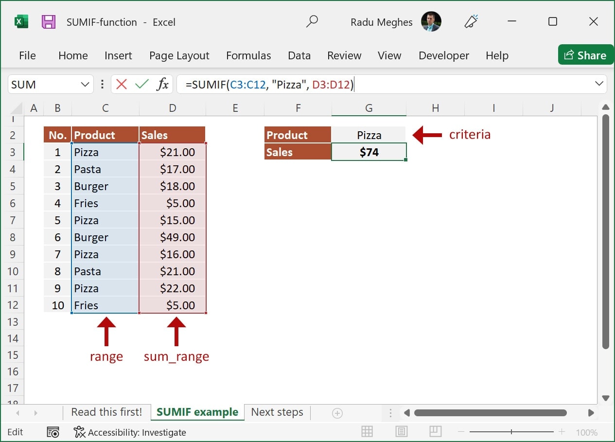
The generic syntax for SUMIF looks like this: = SUMIF ( range, criteria,[ sum_range]) The SUMIF function takes three arguments. The first argument, range, is the range of cells to apply criteria to. The second argument, criteria, is the criteria to apply, along with any logical operators. The last argument, sum_range, is the range that should.
Sum if multiple criteria Excel formula Exceljet
You can use the SUMPRODUCT function and the SUMIF function for adding up values based on multiple criteria. Step-01: Type the following formula in the output cell G8. =SUMPRODUCT (SUMIF (D5:D11,G6:G7,E5:E11)) Here, D5:D11 is the criteria range, G6:G7 is multiple criteria in a range and E5:E11 is the sum range.

Cara Menjumlahkan Data dengan 2 Kriteria Tutorial Rumus SUMIFS YouTube
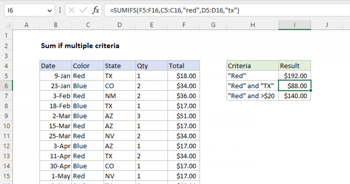
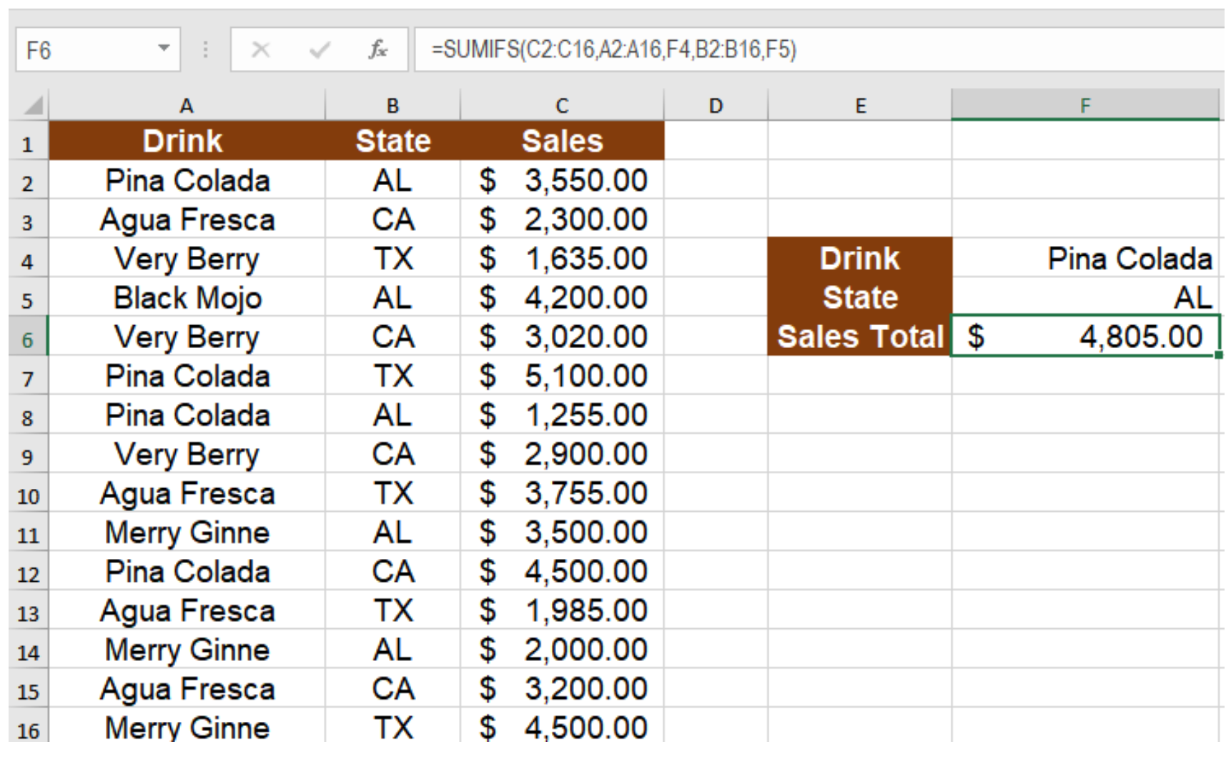
To sum numbers based on multiple criteria, you can use the SUMIFS function. In the example shown, the formula in I6 is: = SUMIFS (F5:F16,C5:C16,"red",D5:D16,"tx") The result is $88.00, the sum of the Total in F5:F16 when the Color in C5:C16 is "Red" and the State in D5:D16 is "TX". Note that the SUMIFS function is not case-sensitive.

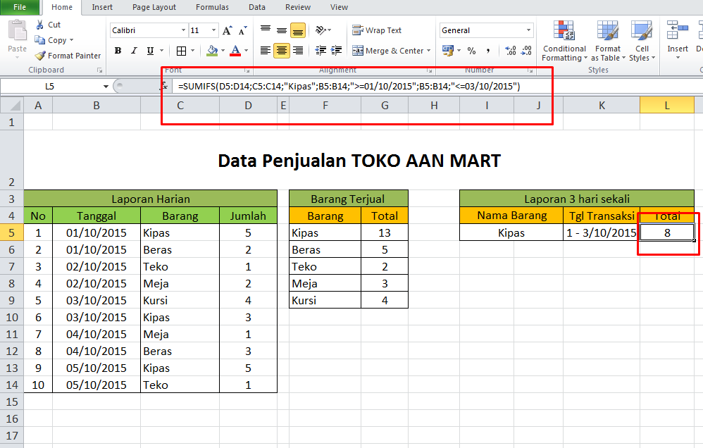
Cara Membuat Rumus SUMIFS (Penjumlahan Rentang dengan 2 dan 3 Kriteria Berbeda) YouTube
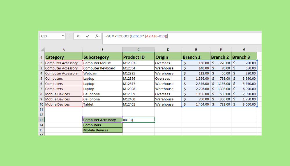
The easiest way to sum multiple columns based on multiple criteria is the SUMPRODUCT formula: SUMPRODUCT ( ( sum_range) * ( criteria_range1 = criteria1) * ( criteria_range2 = criteria2 )) As you can see, it's very similar to the SUM formula, but does not require any extra manipulations with arrays. To sum multiple columns with two criteria, the.

Rumus Sum Sumif dan Sumifs banyak kriteria pada excel YouTube
Suppose you want to sum orders' amounts for either of the products "Orange" and "Apple" supplied as criteria in array constant then you need to provide multiple criteria in SUMIFS function as follows; =SUM (SUMIFS (D2:D22,B2:B22, {"Orange","Apple"})) Remember, you cannot use an expression or cell reference an array constant.

Rumus SUMIF dengan 2 Kriteria YouTube
Begitu juga dengan SUMIF yang ke 2, 3, dan 4 masing-masing menggunakan kriteria >50, D 10 dan >D 10.. Sementara Fungsi SUMIF S dapat menggunakan lebih dari satu kriteria hingga maksimal 127 kriteria dalam satu rumus.Jadi tak heran bila banyak pengguna yang menyebut fungsi SUMIFS sebagai rumus SUMIF bertingkat.
Sumif Excel Example
SUMIF with array constant - compact formula with multiple criteria. The SUMIF + SUMIF approach works fine for 2 conditions. If you need to sum with 3 or more criteria, the formula will become too big and difficult to read. To achieve the same result with a more compact formula, supply your criteria in an array constant:
SUMIFS on Multiple Columns with Criteria in Excel Sheetaki
And click on, Ok. In the functional argument box, select the A2 to A9, Criteria as Ben, and sum range from C2 to C9 and click Ok. This will frame the first half of the multiple criteria syntax. Now insert plus sign (+) as shown below. And click on Insert Function and search for SUMIF and click on Ok, as shown below.
Cara Menggunakan Rumus SUMIF Dan SUMIFS Di Excel Menjumlahkan Data Dengan Kriteria YouTube
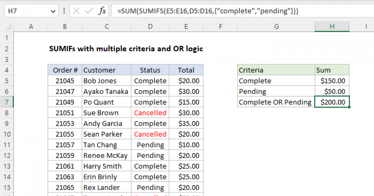
To sum based on multiple criteria using OR logic, you can use the SUMIFS function with an array constant. In the example shown, the formula in H7 is: =SUM (SUMIFS (E5:E16,D5:D16, {"complete","pending"})) The result is $200, the total of all orders with a status of "Complete" or "Pending". Note that the SUMIFS function is not case-sensitive.
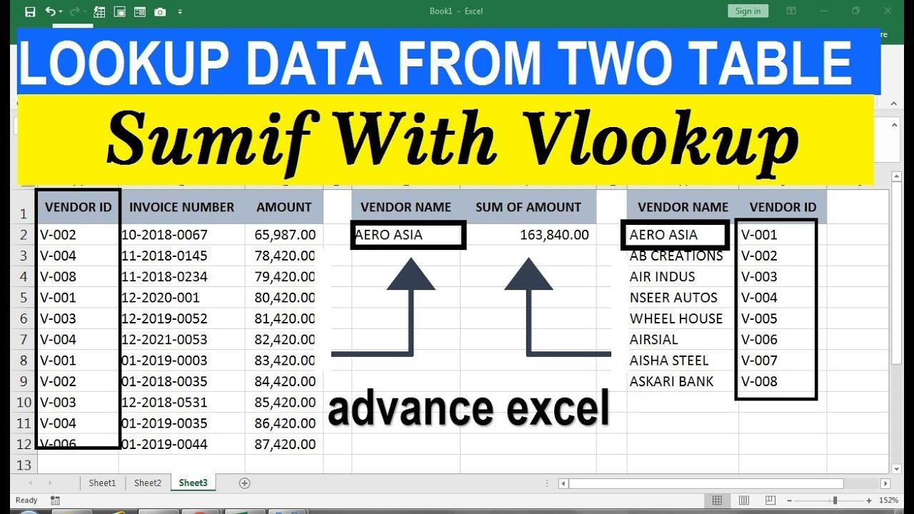
sumif vlookup 2 criteria YouTube
The steps to use the SUMIF with Multiple Criteria are as follows; 1: Choose an empty cell for the output. 2: Type =SUMIF ( select the cell range, enter the first criteria as a cell value or a reference, enter the sum range (optional), and close the brackets. 3: Then press the " + ", and repeat step 2 with new values.
7+ Rumus Sumifs Dengan 2 Kriteria
Anda bisa memasukkan banyak pasangan syarat dengan menggunakan fungsi SUMIFS ini sampai batas tertentu. Pada contoh pertama Penjumlahan akan dilakukan pada kolom JML PENJUALAN (F2:F9) dengan kriteria Kolom Toko (B2:B9) adalah Toko A dan kriteria kedua kolom JUDUL BUKU adalah Buku AB. Baris yang memenuhi syarat tersebut adalah baris dengan nomor.
Rumus Excel Sumif Dengan 2 Kriteria Excel Dan Rumus Microsoft Excel Images and Photos finder
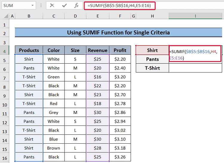
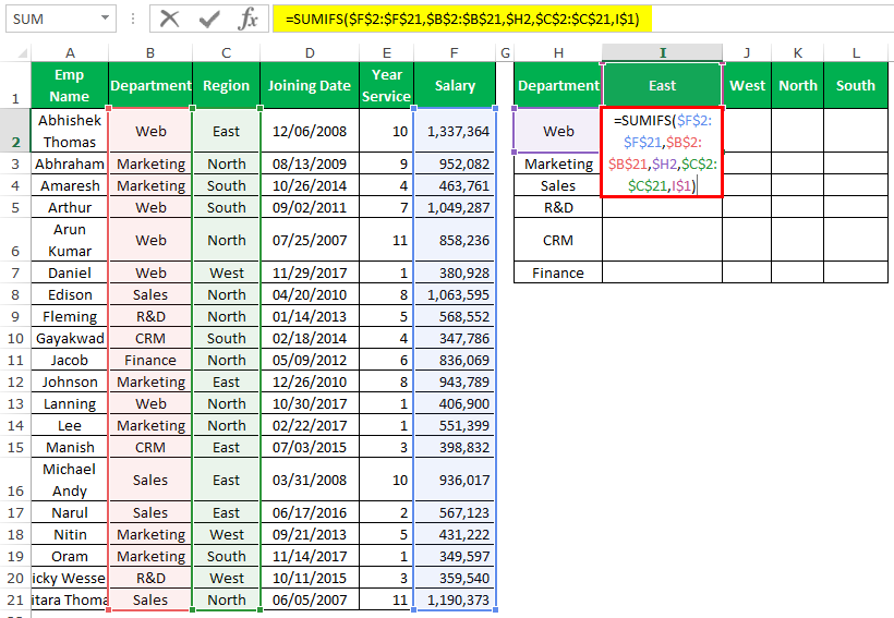
SUMIFS with a cell reference. We can also construct a SUMIFS formula with a cell reference. Let's modify the formula above to use dynamic cells rather than hard-coded values: = SUMIFS (E3:E9, C3:C9, H4, D3:D9, H5) Output: $12,000,000 In the above example, we have replaced our criteria arguments with cell references to dynamic input cells that we've created on the sheet.